On-the-fly projection

On-the-fly projection is one of the many new features in GMS 9.0. On-the-fly projection means that individual objects (coverages, grids, images etc) can define their own projection. If they do, they will be reprojected to a common display projection when drawn. Thus, if you have data defined in different coordinate systems (state plane, UTM etc) you can now import that data as is and it will all be drawn in the right place. The only necessity is that a .prj file accompanies the data or that you specify the projection in GMS after importing.

Objects don't have to define their own projection. If they don't, GMS assumes the object's projection is the same as the display projection and just draws it using the object coordinates without performing any reprojection.

There are a few rules with on-the-fly projection. If an object's projection doesn't match the display projection it cannot be edited. You can, however, change the display projection to match the object's projection, edit the object, and then change the display projection back if you like.

Another rule is that if a grid (2D or 3D) defines it's own projection, the display projection must match the grid projection. GMS will force them to match. Furthermore, all grid objects (2D, 3D and the grid frame) must either define no projection, or all define the same projection.

GUI changes

A number of changes in the GUI were made to support the new projection functionality.

The Projection command was moved from the Edit menu to the Display menu and renamed Display Projection.

The status bar was changed to show the current display projection as well as the latitude and longitude whenever the display projection is a global projection:

Status bar showing lat/lon and current display projection.

A standard "Projection" sub-menu was added to the right-click menu of every object. This menu has commands to set the object's projection, set the display projection to match the object's projection, reproject the object, and transform the object.

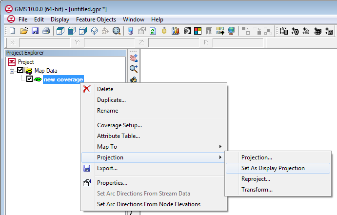
Standard Projection sub-menu added to all objects.

The projection dialog was modified so that it now says "No projection" instead of "Local projection". The difference is subtle, but we felt the new verbage was more accurate.

New Projection dialog.

January 2013 Sprint

• Fixed 8 bugs
• MODFLOW-LGR progress
• PHT3D progress
• MODFLOW-USG progress
• Start of test coverage analysis

December 2012 Sprint

• Added some new images to the Image Gallery
• Released GMS 9.0 out of beta
• Fixed some raster legend issues
• Progress on MODFLOW-LGR
• Progress on PHT3D
• Progress on unstructured grids

Multiple CAD Files

In response to a feature request, starting at GMS 9.0, multiple CAD files can be loaded into GMS at the same time. In the Project Explorer the changes look like this:

Old

New

Also, CAD files are no longer saved when the project is saved. Instead they are treated as externally linked files and only the links are saved.

One other change to CAD file support was the addition of a Properties dialog that shows the CAD file name and path, number of layers, extents, file version, and map projection.

November 2012 Sprint

• Fixed 8 bugs
• Released GMS 8.3.7
• Took GMS 9.0 out of beta. It is now the current version.
• PHT3D support started
• MODFLOW-LGR support - major progress
• Overhauled how framing is done in dev. Framing will be more accurate and the code is much simpler.
• Separated the registry paths for 32 and 64 bit versions in dev
• Created two new transient tutorials for dev
• Wiki -> Help progress
• Added more bitmaps to pop-up menus in dev
• Added basic code coverage analysis for GUI tests

PEST Null Space Monte Carlo

GMS supports multiple methods for performing stochastic simulations such as parameter randomization and indicator simulations. In version 9.0 we have added support for another stochastic method: the PEST Null Space Monte Carlo (NSMC) method. The NSMC method allows you to generate multiple calibrated models with different sets of parameters.

There is always a significant amount of uncertainty associated with a groundwater model.  This uncertainty can be associated with the conceptual model or the field data or the input parameters of the model.  Some model parameters, such as hydraulic conductivity, are particularly prone to uncertainty.  This uncertainty can be reduced by calibrating a model to observation data (monitoring wells, stream flows, etc.).  However, even a well-calibrated model can have significant uncertainty associated with it.

The challenge with a groundwater model is to explore the uncertainty while maintaining a calibrated model (good fit with field measured values). The generation of model input parameters that will respect calibration constraints is a time consuming matter since a parameter estimation exercise must be undertaken for each new set of parameters. However, two tools provided with PEST greatly reduce the amount of time required to perform calibration-constrained Monte Carlo analysis of a groundwater model. The first is the use of SVD-Assist in the calibration process. The second is the pre-calibration null space[1] projection of differences between the stochastic parameter fields and the simplified “calibration parameter field” that is decreed to “calibrate the model”. By using both of these utilities it is possible to obtain parameter sets that respect both the stochastic variability of the subsurface as well as the field measured values; this is accomplished with only a handful of runs per realization.

The results from a PEST NSMC run are illustrated in the figures below where we have two different hydraulic conductivity fields and yet the heads at the observations points remain within acceptable error limits.

Simulation 1 Simulation 2

Using PEST NSMC is very easy in GMS. Two new tutorials have been developed to teach users how to use the NSMC method in GMS. You can find the tutorials in the GMS Learning Center.

---

[1] The null space is comprised of individual parameters, or combinations of parameters, that have no effect on model outputs under calibration conditions. These combinations of parameters can therefore be added to any set of parameters which calibrates the model, to produce another set of parameters which also calibrates the model.

October 2012 Sprint

• Fixed 16 bugs
• Branched GMS 9.0 code base
• Held a GMS training course in Australia
• Initial investigation of MODPATH 6.0 support
• Added a Z Values -> Data Set command for 2D objects
• Changed rasters so that interpolation using a raster catalogs results in one data set and interpolation from multiple selected rasters results in multiple data sets
• Unstructured grids are now rendering in GMS
• Cleaned up a lot of help links on the wiki and help buttons in GMS
• Switched scatter points to use the standard Contour Options
• Added exporting of 3D grids to a VTK file for use in ParaView
• Progress on support for multiple grids
• Progress on wiki to dynamic help file